Customising plots with ggplot2

library(ggvariant)
library(ggplot2)

vcf_file <- system.file("extdata", "example.vcf", package = "ggvariant")
variants <- read_vcf(vcf_file)
#> ℹ Reading VCF: example.vcf
#> ✔ Reading VCF: example.vcf [24ms]
#> 
#> Loaded 19 variant records across 7 chromosomes.

Every ggvariant plot function returns a standard ggplot object (not a subclass, not a wrapped list), so any ggplot2 layer, scale, theme, or annotation composes onto it exactly as it would onto a plot you built by hand.

Adding layers

plot_lollipop(variants, gene = "KRAS") +
  labs(subtitle = "KRAS mutations in cohort X") +
  theme(legend.position = "bottom")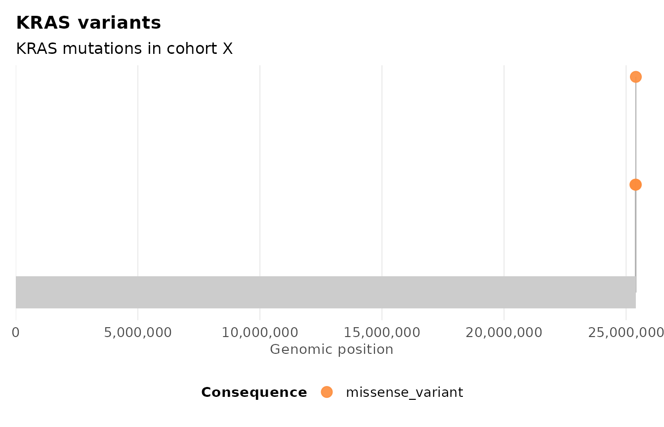

Overriding a scale

ggvariant sets a fill or colour scale internally, so replacing it means adding a new scale_* call after the plot is built – ggplot2 uses the last matching scale in the layer stack.

plot_consequence_summary(variants) +
  scale_fill_brewer(palette = "Set2", name = "Consequence")
#> Scale for fill is already present.
#> Adding another scale for fill, which will replace the existing scale.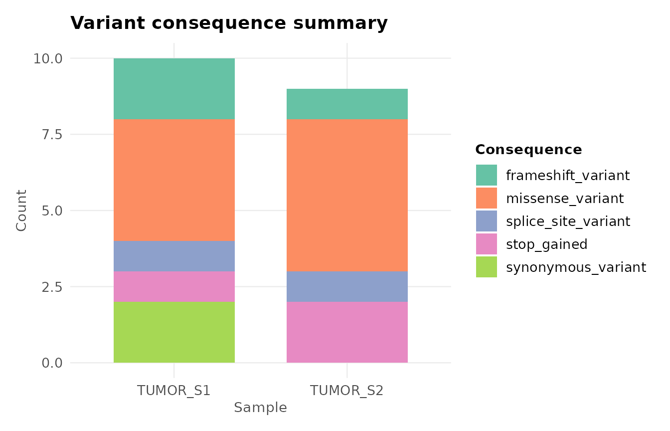

Building on theme_ggvariant()

theme_ggvariant() is exported, so you can start from it rather than theme_minimal() when building a custom plot from scratch, or layer further theme() tweaks onto a ggvariant plot’s existing theme.

plot_variant_spectrum(variants) +
  theme(
    axis.text.x = element_text(angle = 45, hjust = 1),
    plot.title  = element_text(colour = "grey20")
  )
#> Excluded 2 non-SNV records from spectrum plot.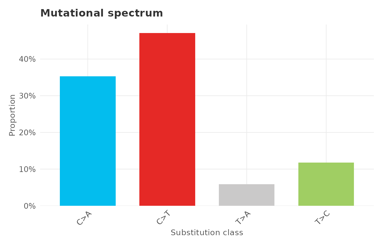

Combining with gv_palette()

The built-in palettes are exported as plain named character vectors, so they work equally well outside a ggvariant plot function – for example, when building a custom ggplot2 call directly against a gvf object.

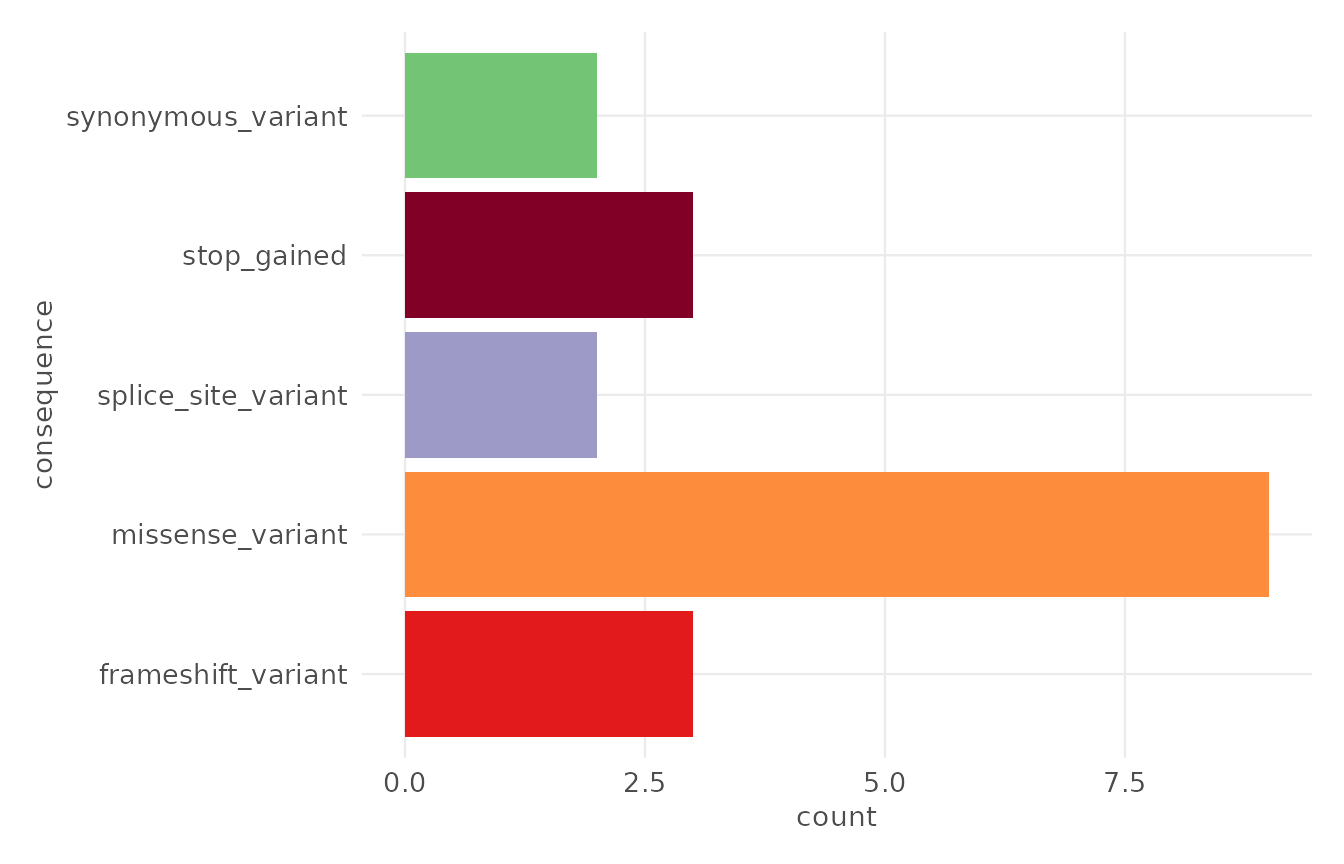
ggplot(variants, aes(x = consequence, fill = consequence)) +
  geom_bar() +
  scale_fill_manual(values = gv_palette("consequence"), guide = "none") +
  coord_flip() +
  theme_ggvariant()